Do you need to add a custom field in your Pivot Table? You want to create an additional calculated field but you don’t know how to do it? No worries, Ted Jordan is here to help!
At first, using a Pivot Table in Excel or in Google Sheets can seem tricky but you will discover that adding a new calculated field is pretty easy. Follow our tutorial to add, personalise and use calculated fields in your Pivot Tables. For Excel or Google Sheets, we created an easy guide just for you!
Calculated fields in Excel
How to add a calculated field in your Excel Pivot Table
Once your Pivot Table is created in Excel, follow these straightforward steps to create a new calculated field.
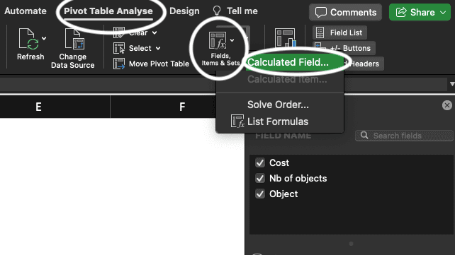
– Click on your Pivot Table: the Pivot Table Analyse tab will appear on top the Excel window.

– Click on Pivot Table Analyse>Fields, Items & Sets>Calculated Field…
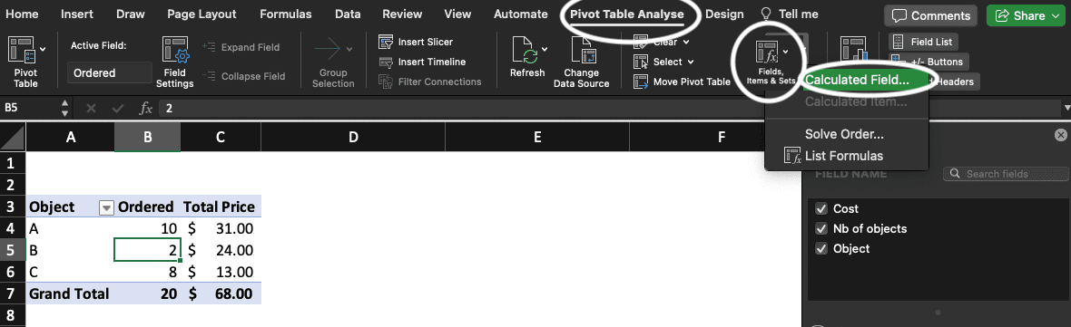
– After clicking on Calculated Field, a window will pop up: Insert Calculated Field.
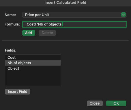
Name: enter the name of the new field.
Formula: enter the formula of your calculated field.
Two ways of doing it:
Double-click the name of the fields you want to use and add manually mathematical signs.
OR
Select each field you need for the formula and click “Insert Field”, then add manually mathematical signs.
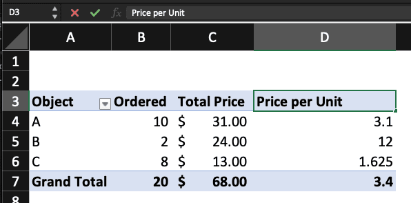
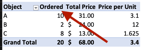
In this example, we want to create a calculated field in our Excel Pivot Table, to calculate the price of each object, per unit. We call it “Price per Unitâ”and the formula is Price per Unit=Cost/’Nb of objects’.
– Click OK and the new calculated field is now appearing in your Pivot Table.
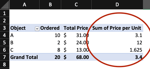
You may have noticed that the names of our existing fields and the new calculated field are different too. We did change their names; also the name of the new field is not what we want to use.
In order to modify the name of a field in a Pivot Table, check the steps below or go directly to Field Settings (Pivot Table Analyse>Field Settings).
How to modify a calculated field in your Excel Pivot Table
There are various ways of changing the name of a field in Pivot Tables, here are two:
Example 1 – Changing a field name in Excel
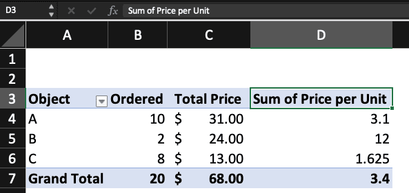
In your Pivot Table, click the cell you want to modify and type directly its name.
>>>
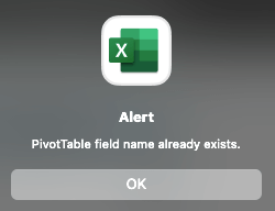
If you use a field name which existing exists, you will have an alert message like this one:
Example 2 – Changing a field name in Excel
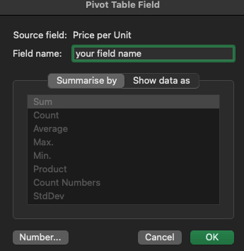
In your Excel Pivot Table, double-click the cell containing the name you want to modify: a window will pop up “Pivot Table Field“. Change the field name directly in it and click OK.
What’s the difference between Source Field and Field name in Excel?
The Source Field is the name of a field in the source data (for example, the data selected to create your Pivot Table).
Meanwhile, the Field name corresponds to the name shown in your Pivot Table for a specific field.
For example, in our case, Source Field is “Nb of objects” and Field name is “Ordered”. “Nb of objects” is the name used in our source data while “Ordered” is what is shown in our Pivot Table.
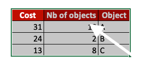
Source data
Field name
Now that the names are changed in your Pivot Table, maybe you noticed an error in the formula you entered for your calculated field? If you want to change the formula of your calculated field, go back to the Calculated Field window.
How to change a calculated field formula in Excel?
To correct the formula of one of your calculated fields, go back to Pivot Table Analyse>Fields, Items & Sets>Calculated Field…
When you see the Insert Calculated Field window, select the Field you want to modify by clicking the green arrow.
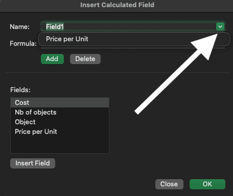
You can now change the formula and click OK or Modify to save the changes you made.
We do recommend to add IFERROR in your formula so your Pivot Table will not contain any error messages. To learn how to use the IFERROR function in Excel, check this tutorial.

Calculated fields in Google Sheets
How to add a calculated field in your Google Sheets Pivot Table
Adding a new calculated field in your spreadsheet is easy! Once your Pivot Table is created, click the Edit button.
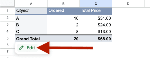
The Pivot table editor window will open; then click Add and select Calculated Field to add a new field to your Pivot Table.

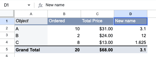
Now enter the formula you want to use for your calculated field. Note that if you enter a name with more than one word, you have to use ‘‘ or the formula will be incorrect.

Your calculated field formula is entered and you can see the new field in you Pivot Table but you want to change its name? Just change its name directly in the Pivot Table!
How to change a calculated field name in Google Sheets
In order to modify the name of a field in your Pivot Table, just click the cell with the name you want to change and type the new name you wish to use.
Now, you know how to add calculated fields in Pivot Tables!
Discover more tutorials to become a MS Excel expert: IFNA function, IFERROR function, VLOOKUP, etc.