Do you wonder what are the unique values in your Excel table? Do you need to extract unique data or remove duplicate values? Have you ever heard of the UNIQUE function in Excel?
The UNIQUE function returns a list of unique values in a specific list or in a range. This function is handy when you want to extract unique data from long lists for example.
What’s the UNIQUE formula in Excel?
The UNIQUE formula syntax in Excel is =UNIQUE(array,[by_col],[exactly_once]).
It contains 1 required argument and 2 optional ones.
array – the range or array to analyse. It can be rows, columns, or a combination of both. This argument is required.
[by_col] – (optional) This is a logical value indicating how to compare the data in array. TRUE compares columns against each other while FALSE (or omitted) compares rows against each other.
[exactly_once] – (optional) This argument returns rows or columns that occur exactly once in the array argument. It’s a logical value: TRUE or FALSE. TRUE returns all unique values in rows or columns occurring just once within the array argument. FALSE (or omitted) returns all distinct rows or columns from the array argument.
How to use the UNIQUE function in Excel
To use the UNIQUE function in Excel, first decide which array to analyse. Then, decide where you want the result to appear, knowing you will need some blank cells (in rows and in columns sometimes).
The error message SPILL! will appear if you don’t leave enough space (blank cells) for the UNIQUE results.
To find unique values on Excel, adapt the UNIQUE formula to your request. Check the various examples below to learn from them and easily find unique values!
Find unique values in a row
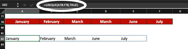
To find unique values in a row, in Excel, use this formula: =UNIQUE(array,TRUE).

In this example, we want to display unique names (there is an extra “March”).
Find unique values in a column
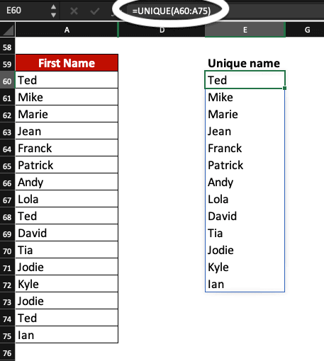
In Excel, find unique data in a column by using the following formula: =UNIQUE(array).
In this example, we want to find unique names from our customer list. All the names are in column A, from cell 60 to cell 75. The formula we use is =UNIQUE(A60:A75).
As a result, Ted and Jodie only appear once in the new list.
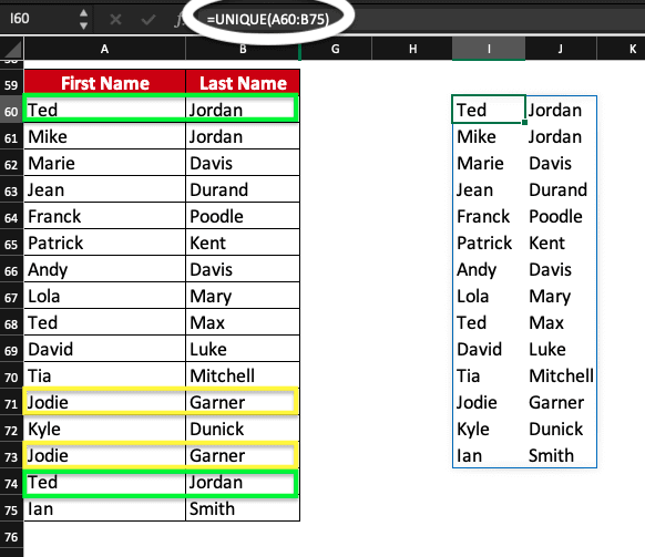
Find unique values within a table
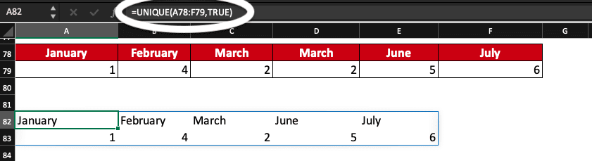
If you have some data linked between rows and columns in a table and want to find unique values, in Excel use this formula: =UNIQUE(array,TRUE).
Note that if you have a vertical table, you can just use write =UNIQUE(array) for the UNIQUE function.

In this example, we want to delete duplicates (indeed, the column March with the number 2 is appearing twice).
In this other example, we want to delete duplicated customers. Indeed, Ted Jordan and Jodie Garner appear 2 times in our table.
We used the formula =UNIQUE(array) but could have also used =UNIQUE(array,TRUE) because this is a vertical table.
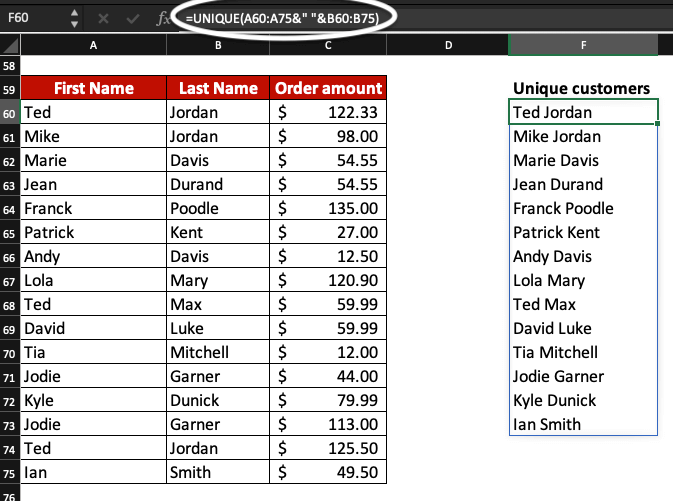
In the above example, first and last names are detached because they are written in 2 different columns. This might be confusing to read because some customers share the same first name (Ted Jordan and Ted Max) or last name (Ted Jordan and Mike Jordan). If we want the result to show full names within the same column, we just need to add ampersands (&) within the UNIQUE formula.
The formula is =UNIQUE(data_in_column1&” “&data_in_column2) so =UNIQUE(A60:A75&” “&B60:B75).
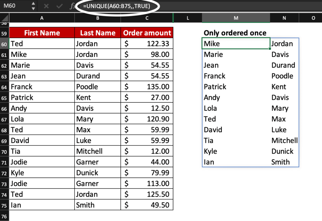
One-time only values in Excel
Finding a unique value in Excel might not be enough for your request. If you need to find unique values appearing only once in a row, a column or in a table, just add TRUE to the least argument.
Find unique values (appearing only once) by using the UNIQUE formula =UNIQUE(array,[by_col],TRUE).
For example, we want to find customers who ordered with us only once, from our customer list. We want to find their name and send them a promotional code so they would make more purchases.
We are comparing rows against each other in our table (vertical table) so we can type =UNIQUE(A60:B75,,TRUE) or =UNIQUE(A60:B75,FALSE,TRUE) as the UNIQUE formula, for this example.
Thanks to this tutorial including various examples, now, you know how to find unique values in Excel.
Extracting unique values and filtering duplicates out in Microsoft Excel is now a new skill of yours!
Do you know you can receive an Excel certificate to add to your CV or LinkedIn profile thanks to Ted Jordan? To do so, click here!