Conditional formatting is a great way to distinguish data in your Excel table!
Learn how to create a rule in Excel to change cell colour based on value (numbers or text). Use conditional formatting with the IF formula or else and understand your worksheet data within seconds.
Highlight percentage of completion or the highest value in a column with this handy tool!
Ready to use cell formatting in MS Excel?
What is conditional formatting?
Conditional formatting: a rule created with one or multiple conditions dictates the format of a cell or its content (for Excel).
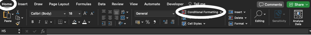
Where is conditional formatting in Excel?
Find the conditional formatting menu in the Home tab in Excel.
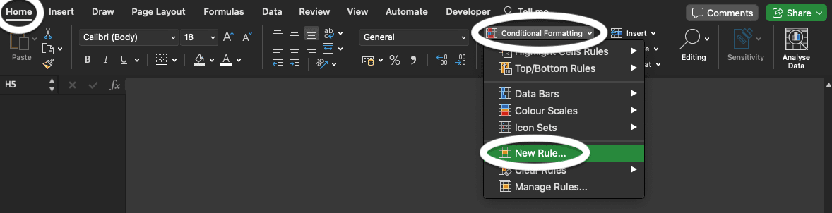
How to create a rule in Excel?

In Excel, create a new rule for conditional formatting by selecting Home, Conditional Formatting then New Rule… or you can use existing templates (greater than, top 10%, etc.).
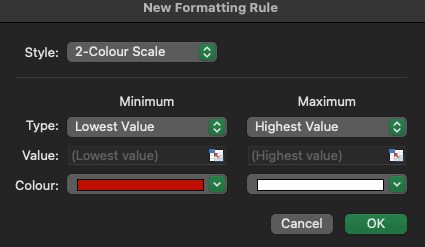
The New Formatting Rule window will appear; you can now create your own rule.
Check the examples below to learn how to create rules for text and values.
Change cells colour based on value

In this example, we want to change cell colour based on value. We aim to colour code cells to highlight youngest and oldest persons.
We decide to use colour scales, with cells containing the highest numbers being highlighted in red (vs white for the youngest ages).
If you want to change colours, click Conditional Formatting then Manage Rules. Select the rule you want to edit by double-clicking it or by selecting it then clicking Edit Rule…
Conditional formatting based on text
Use conditional formatting in Excel to highlight cells containing specific words for example or client names.
In this example, we want to colour cells containing email addresses in “.org” in blue and the ones in “.com” in yellow.
Note that you can change only the text colour if you want, or mix text colour and cell colour, change text to bold, etc.
Conditional formatting with the IF formula
Many of our students ask how to use conditional formatting with the IF function in Excel. There are plenty of ways of doing it but here is one example of conditional formatting and IF used together.
In this example, the IF formula is =IF(F2=TRUE,”Yes”,””) for row 2, =IF(F3=TRUE,”Yes”,””) for row 3, etc.
We want “Yes” to be written in green for IF=TRUE and the cell to be coloured in red for “IF is not TRUE”.
Watch our 50 sec. video and create rules for conditional formatting within seconds in the future!
Now, our Excel table is responsive!
Check this free tutorial if you need a refresher for the IF function and click here to learn how to create checklists in Excel!
Now, you know how to find, create, edit conditional formatting in Excel and increase the level of professionalism of your Excel worksheets. You can change cell colour based on value or text.
FREE – No credit card needed