Tired of using the good old filters in pivot tables? Do you want to filter out your tables quickly? Try slicers!
Slicers are great to filter data in tables like pivot tables or regular ones. They decrease risks of making mistakes when ticking filter options and save you time. Learn how to add slicers in Excel by checking our tutorial below!
Adding slicers in Excel will become a new habit to finish projects earlier. Also, your colleagues or customers will be happy to select the data they need directly without the need of using regular filters. Ready to learn?
How to insert slicers in Excel
Adding slicers to a pivot table in Excel
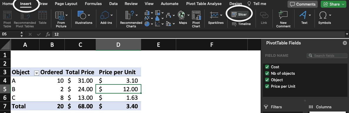
On Excel, click anywhere in your pivot table then go to Insert>Slicer.

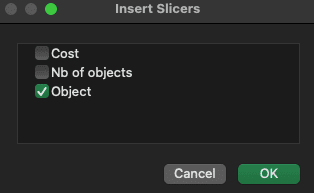
Now that the Insert Slicers window is visible, select the filter category you want to use (you will be able to rename it later) and click OK. If you tick several filters, you will have several slicers in your worksheet.
You just added a slicer to your pivot table!
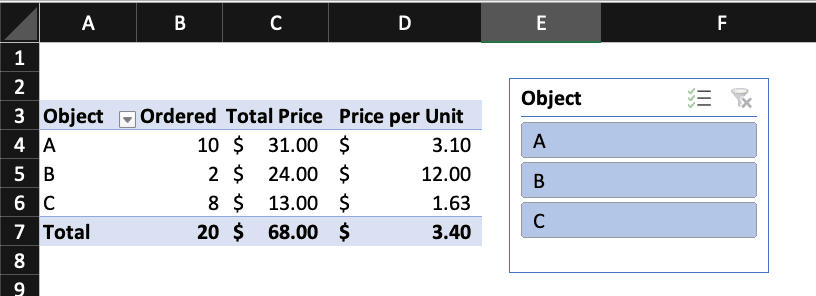

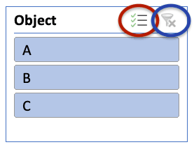
Click on any option to filter your pivot table easily and quickly. If you want to select multiple options, click first on the Multi-Select icon (in red). And if you don’t want to apply filters anymore on your Excel pivot table, click Clear Filter (in blue).
Adding slicers to a table in Excel
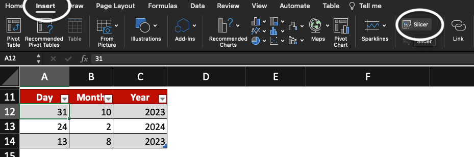
Creating a slicer for a table in Excel is easy. Click on your table then go to Insert>Slicer.
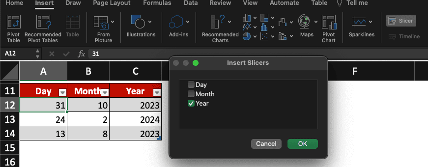
Select the field you want to use as filter and click OK.
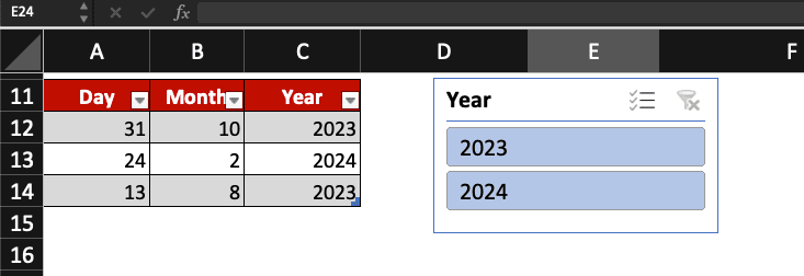
You just added a slicer to your Excel table! Now click one of the filter options, you are ready to work quicker.
>> Did you know you could create a table just by selecting cells in Excel and pressing Command+T keys? Now you know!
Do you want to change the Excel slicer design to match your brand colours or tables? Check how to do it below.
Excel slicers design: how to change it?
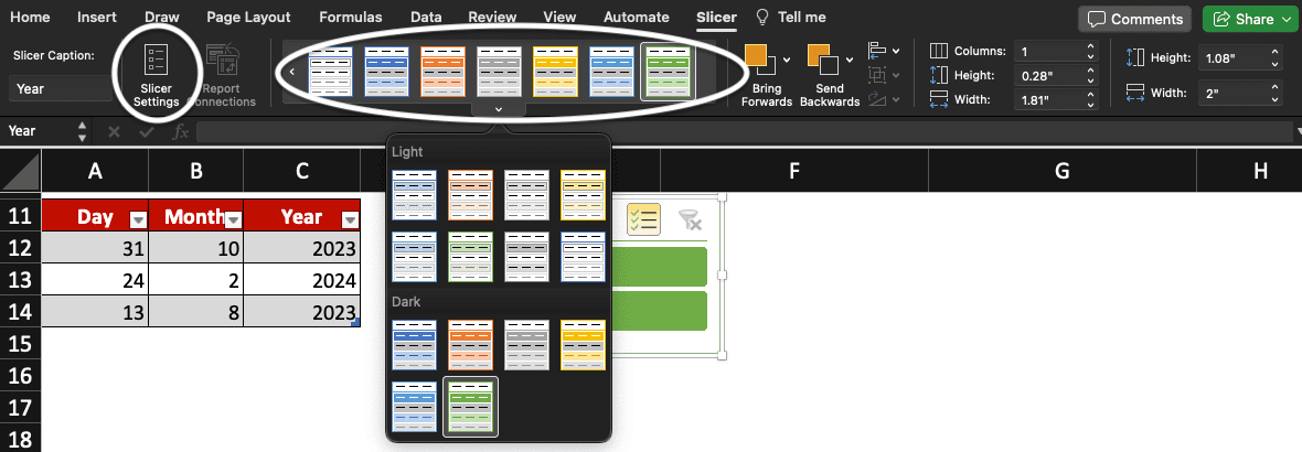
You can find Slicer Settings or change slicers design in the Slicer tab. You can also change the slicer caption by a more appealing name if you wish (top left corner of the Slicer tab).
Change the design of your slicer by selecting a light or dark design; just click the one you want to use. You can also change columns number on the right of the tab, which can offer a better design for your Excel spreadsheet.
If you want to learn more Microsoft Excel tricks, check our blog or join our Certifying Course now!