Gauge charts are great to quickly see how well a metric is performing against a target goal. For example, managers use them during performance reviews, analysts and account managers during client meetings.
But this handy tool is not easy to find in Excel. Why is that?
Discover our tips and tricks to create gauge charts in Excel. Even for beginners!
Ready to learn a new skill?
Is there a gauge chart in Excel?
No, Microsoft Excel does not offer gauge chart templates for now, despite a large selection of charts to use.
So, is there a gauge chart alternative in Excel?
There is better than that: you can use doughnut charts to create gauge charts!
From doughnut chart to gauge chart
Create gauge charts in Excel by customising doughnut charts in only 3 steps! You just need to twist some parameters to end with the result you want.
Before creating a doughnut chart, make sure to add the total amount of the values you will use.
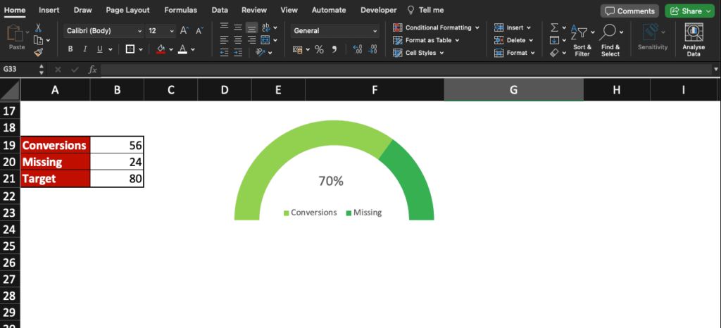
For example, let highlight the number of conversions made compared to a target.
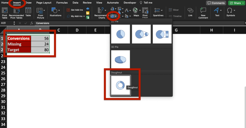
In your Excel table, make sure to add the conversions (56), the number of conversions missing to reach the target (24) and the target (80).
How to create a doughnut chart
To create a doughnut chart in Excel, start by selecting your data then go to Insert, click the Pie selection and select Doughnut.
Your doughnut is created, it’s time to transform it into a gauge chart!
Gauge chart in Excel
Create a gauge chart in Excel by following the steps below:

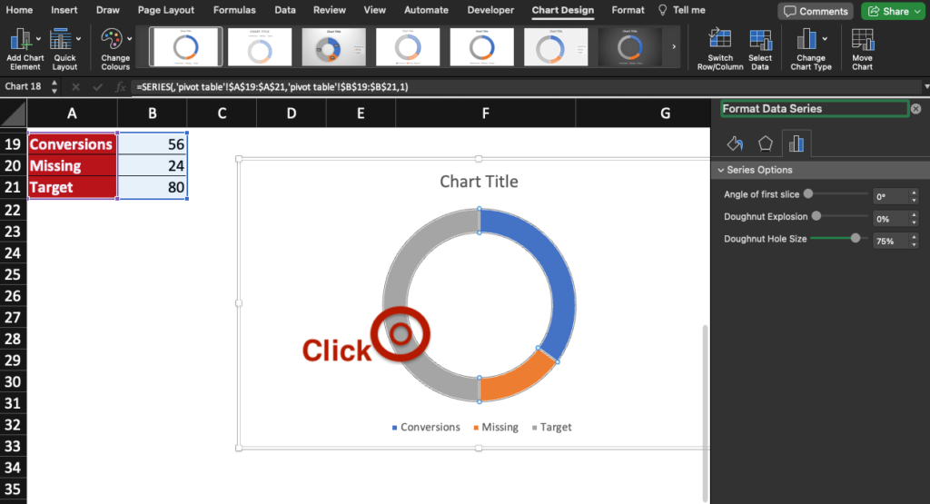
- Double-click the doughnut you just created: the Format Data Point will appear.
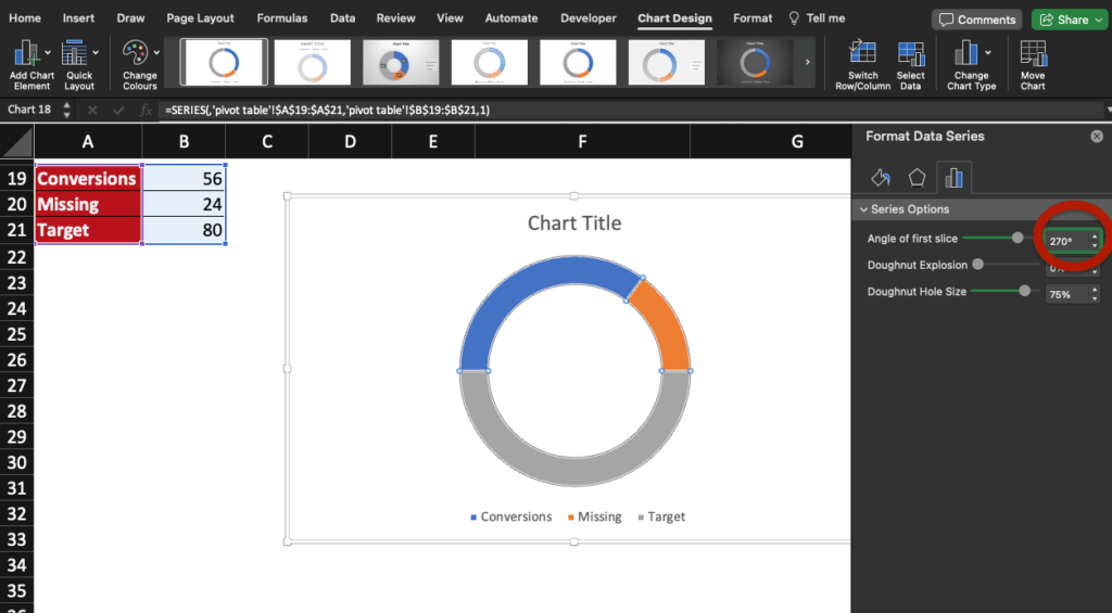
- Set the angle of first slice to 270°.

- Select the bottom part of the doughnut (in grey here), go to Format Data Point and select No fill.
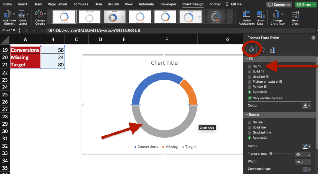
You now have a simple gauge chart in your Excel worksheet!
For a professional look
Follow some of these extra steps to customise your chart for a professional look:
- Delete the legend of the unseen part (Target in our example) by selecting it and pressing the delete key on your keyboard.
- Customise the chart title with key data such as the percentage of completion and place it in the centre of your chart.
- Set the border of your gauge chart to No line.
- Move the legend inside the chart.
- Change the colours of the shape elements.
- Etc.
And now you have it: a simple but impressive gauge chart in Excel.
Now, you know how to create a gauge chart in Excel and how to customise it.
What will you learn next? Check our blog for more tutorials.