To create a checklist in Excel you may want to insert multiple checkboxes: learn how to add tick boxes with this quick tutorial.
Before showing you how to create a checkbox in Excel, let us show you where to find the checkbox tool. The easiest way to insert a tick box in Excel is to do it via the Developer tab.
Where is the developer tab in Excel?
In Microsoft Excel, add the developer tab by following these quick steps:
- Click Microsoft Excel > Preferences.
- Click View.
- Select Developer tab under In Ribbon, Show.
Now that you know how to enable the Developer tab in Excel, let create a checklist together. Let insert a checkbox in Excel!
How to insert a checkbox in Excel?

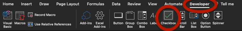
To insert a checkbox in Excel, go to the Developer tab and click Checkbox.
After clicking Checkbox, click on your Excel worksheet: a checkbox is now created! Now, let customise it.
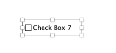

We recommend deleting its name so only the tick box is visible. To do so, click directly on its name or change its name on the top left corner (next to formula).
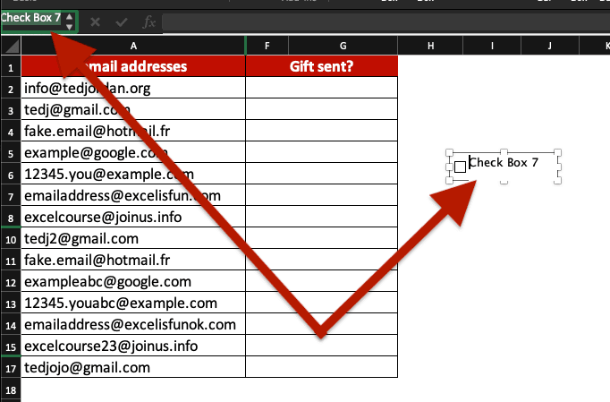
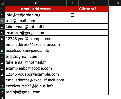
Now drag the checkbox to the cell you want. In our example, we want to create a checklist and tick boxes when a gift has been sent to our most loyal customers.
How to insert multiple checkboxes?
Inserting a checkbox in Excel is quite simple and quick but if you need multiple checkboxes in Excel, this might take a while… Save time by copy-pasting the checkbox you just created by performing a drag and drop with a right click, as many times as needed.
You can also select multiple checkboxes and copy-paste several at a time.
Now that you have all the tick boxes created for your Excel checklist, how to align them?
How to align checkboxes in Excel?
To align checkboxes in Excel, follow these 4 quick steps:
- Select all your checkboxes;
- Click Shape Format;
- Click Align;
- Select the alignment you want.
We could stop here and just tick boxes if a gift has been sent to each specific customer. Because it can be difficult to differentiate ticked and unticked boxes in Excel, when you have a lot of data, we recommend to spend a few more minutes customising the checklist.
How to add text when we tick a box in Excel?
To link a cell to a tick mark box, perform a right click on the box and select Format control. Then enter a value for cell link.
In our example, we want to link the tick box with cells in column F. For the checkbox in cell F3, the cell to link will be F3; for the one in cell F4, the cell to link will be F4, etc.
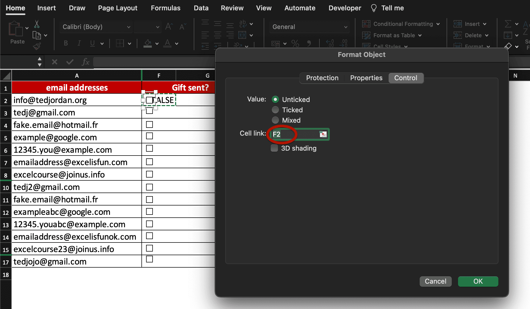
We could stop here as TRUE will appear when a box is ticked and FALSE when it isn’t.
We want to customise our table so text only appears when a box is ticked. To do so we use the IF function; here are the steps to follow:
- Select the cells where TRUE/FALSE messages appear and change the text colour to white. Now we can’t see the text when we tick or untick a check box.
- Enter =IF(F2=TRUE,”Yes”,””) in the G2 cell (it could be any cell but in our example we want to use this one).
- Apply the same formula to other rows and enjoy your new clear checklist!
Now, you know how to create a tick box or checkbox in Excel and how to customise a checklist.
Join our online Excel Course and become a Spreadsheets Master!