Discover the Excel AutoSum shortcut and use AutoSum like a pro with Ted Jordan.
Sum Excel columns and rows quickly with this handy tool!
Ready to learn how to use AutoSum?
What is AutoSum in Excel
AutoSum is an Excel tool that sums a range of cells together and displays the result after the selected cells. It can be used to calculate a sum, an average value or even to display the maximal value of a column.
Where is AutoSum in Excel
You can find AutoSum by clicking Home then AutoSum or in the Formulas tab. The tool is represented by the Greek uppercase Sigma symbol Σ.
You may use the AutoSum shortcut to sum your data quicker.
What’s the Mac AutoSum shortcut?
For Mac users, the AutoSum shortcut for Excel is Command + Shift + T.


How to use AutoSum in Excel
Like we said, you can use AutoSum to sum a column of numbers. By default, the formula applied by AutoSum is SUM.
To sum a column of numbers, select the cell just below the last number of the column then press Command, Shift then T.
Sum a row of numbers by selecting the cell just after (to the right) the last number of the row then press Command, Shift then T.
Check our examples below to understand how it works even better.
Example – Sum of column
In this example, we want to calculate the sum of all orders, for each quarter.
First, we select the cells where we want the results to appear (just below the last number of each column).
Then, we press Command, Shift then T and voilà !
Example : Maximal value in a row
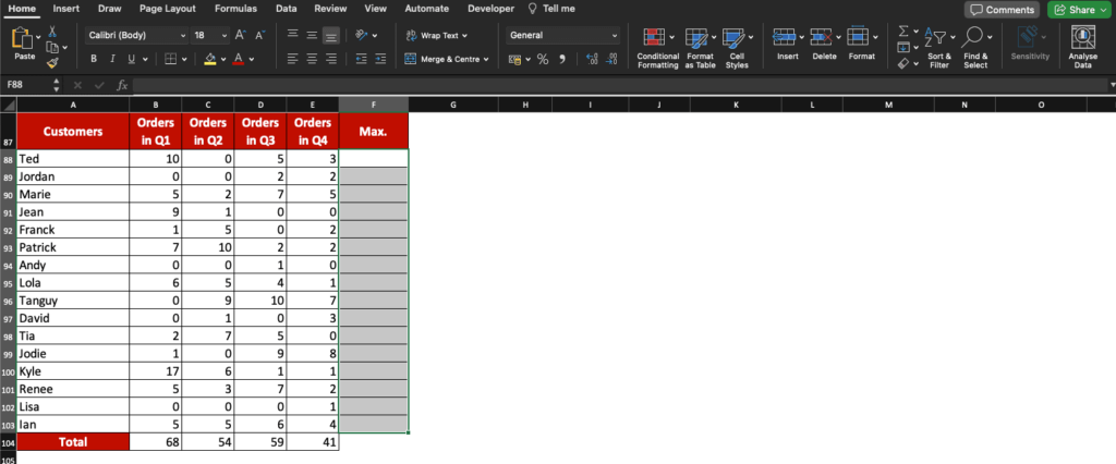
In this example, we use AutoSum to know what’s the maximal number of orders each client purchased with us during the year.

We start by selecting the cells directly on the right of the last number of each row (F88 to F103).
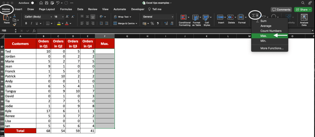
We then find AutoSum in Home>AutoSum and click the option button to select Max.
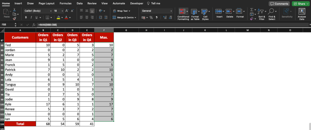
The max. value for each row now appears at the end of each row.
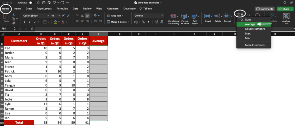
Example – Average value in a row
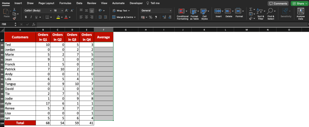
To know what’s the average number of a row, use Excel AutoSum tool. In this example, the goal is to calculate the average number of orders per customer.
Select the cells directly on the right of the last number of each row (F88 to F103).
Click the option button next to the Sigma symbol in the Home tab and select Average.
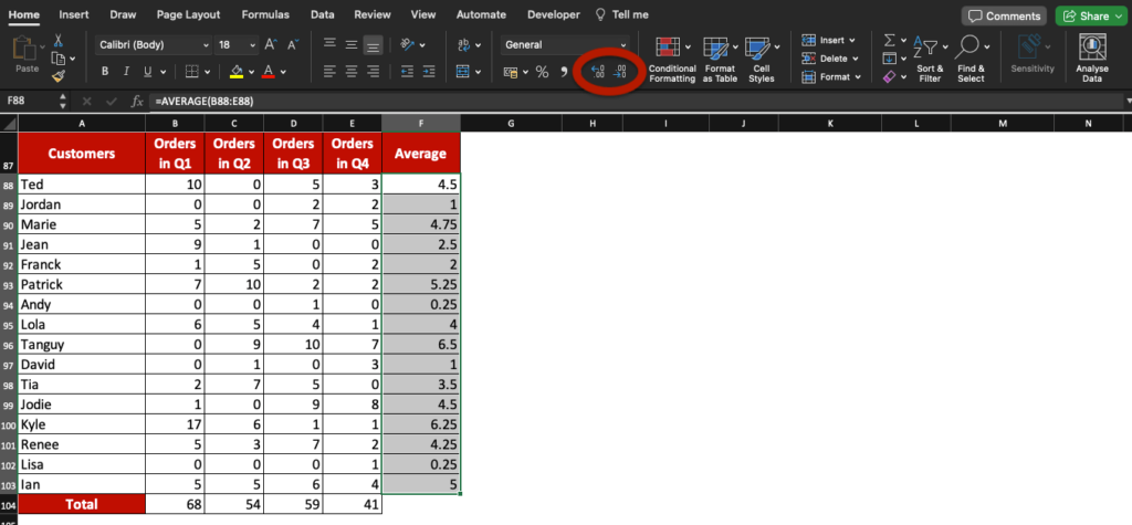
You now see the average number of orders for each of your customers. Use the indent function (highlighted in red here) to format numbers.
Now, you know how to use AutoSum in Excel and what the AutoSum shortcut for Mac is!
Learn more tips for becoming a Spreadsheet Pro with our free Excel Online Course. Learn at your own pace!