Use SUMIFS in Excel instead of VLOOKUP when you need to check multiple criteria before calculating a value.
In this free Excel tutorial, learn what SUMIFS does and how to use it between dates for example.
Did you know you can add up to 126 additional criteria if needed?
SUMIFS function in Excel
SUMIFS will result in a number, the sum of the arguments meeting multiple criteria, within a range.
In Excel, SUMIFS is the equivalent of the SUMIF function with multiple criteria.
In Excel, the SUMIFS formula is =SUMIFS(sum_range, criteria_range1, criteria1, [criteria_range2, criteria2], …). It contains 3 required arguments.
sum_range — the range of cells to sum.
criteria_range1 — the range where the first criteria is checked.
criteria1 — the first criteria checked, defining which cells will be added from criteria_range1.
SUMIFS function tips
– Enclose text criteria or criteria with logical/mathematical symbols in quotation marks (“text”).
– You may use wildcard characters in criteria arguments. A question mark (?) will search for any single character and an asterisk (*) will match any sequence of characters.
SUMIFS between two dates
Use the SUMIFS function to sum data between two dates. Learn how to do it by following these steps:
- Enter =SUMIFS( in the cell where you want the result of the formula to be displayed
- Add the range of cells to sum followed by a comma (,)
- Enter the range where dates appear followed by a comma(,)
- Enter “>=dd/mm/yyyy“, with dd/mm/yyyy being the oldest date in your time range
- Again, add the range where dates appear followed by a comma(,)
- Then, enter “<=dd/mm/yyyy“) with dd/mm/yyyy being this time the most recent date in your time range
- Finally, click Enter.
Example — Sum between two dates
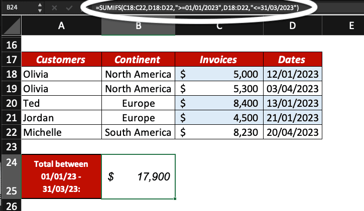
In this example, we use SUMIFS between two dates to calculate the invoices total during a specific time range (01/01/2023 to 31/03/2023 included). We highlighted the dates and invoices following our criteria in blue for your convenience.
The formula we use is =SUMIFS(C18:C22,D18:D22,”>=01/01/2023″,D18:D22,”<=31/03/2023″).
C18:C22 corresponds to the range of cells containing invoices values.
D18:D22 corresponds to the range where dates appear.
Example — SUMIFS with 3 criteria

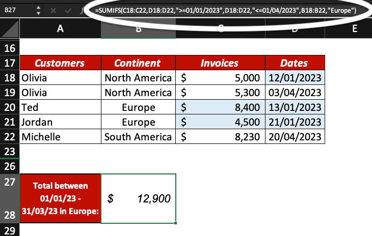
In this example, we use the SUMIFS function to calculate the invoices total during a specific time range (01/01/2023 to 31/03/2023 included), from our customers based in Europe. We use 3 criteria in our formula.
For clarity, we highlighted the dates and invoices following our different criteria in blue.
The formula we use is =SUMIFS(C18:C22,D18:D22,”>=01/01/2023″,D18:D22,”<=01/04/2023″,B18:B22,”Europe”).
C18:C22 corresponds to the range of cells containing invoices values.
D18:D22 corresponds to the range where dates appear.
B18:B22 is the range of cells where the criteria Europe is applied.
Now, you know what the difference between SUMIF and SUMIFS is in Excel and how to use the latter.


2 responses
glad to be one of the visitors on this awing site : D.
Oh my goodness! Impressive article dude! Thank you so much, However I am encountering difficulties with your RSS. I don’t understand the reason why I cannot subscribe to it. Is there anybody having the same RSS problems? Anybody who knows the answer will you kindly respond? Thanx!!