Learn how to write AND function in Excel like a pro with Ted Jordan: discover the AND function formula, how to use it with multiple criteria or text and when to use it.
Read our tutorial to understand how the Excel AND function works in various situations.
Ready to increase your Excel knowledge?
Let’s go!
Excel AND function
The Excel AND function determines if all conditions included in its syntax are met: if so, TRUE will appear as the result of the AND formula. If not all conditions are met, FALSE will be displayed.
Excel AND function formula
The Excel AND function formula is =AND(logical1, [logical2], …) with logical1 being the only required argument.
logical1 — this argument represents the 1st condition you want to test with the AND formula.
logical2… — additional conditions to test with the AND formula.
Excel AND function – Tips
– You can add up to 255 conditions in the AND function in Excel.
– Empty cells will be ignored by the system.
– For conditions with text elements, use quotation marks “” in logical values or the system will skip these cells.
When to use the AND function in Excel
We recommend to use the Excel AND function when you want to test multiple conditions at the same time.
To display specific values for TRUE or FALSE result, you can combine AND with IF for example.
How to use the AND function
Use the AND formula in Excel when you want to check if some conditions are all met. You can of course use AND for 1 condition if you wish to, or use this handy function with IF to display specific results.
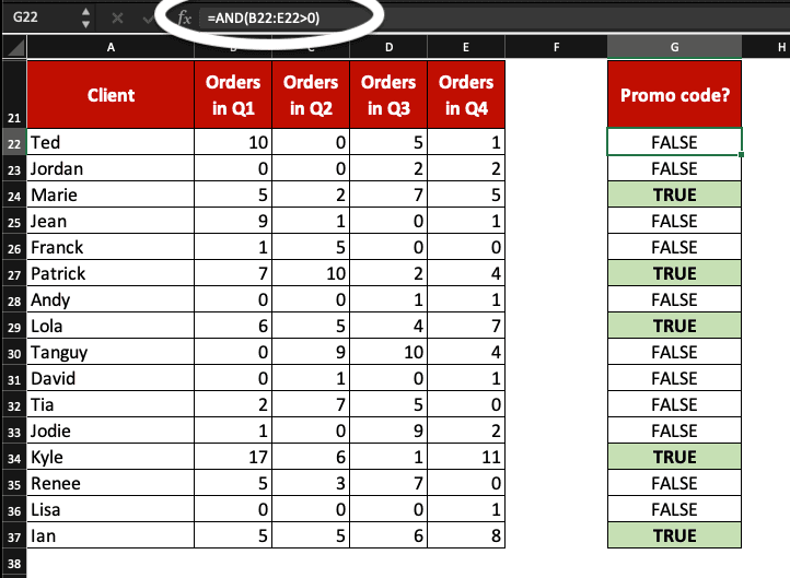
AND function with 1 criteria but multiple cells: how to do it?

You can test one criteria (condition) in Excel for multiple cells easily with the AND function.
For example, =AND(B22:E22>0) will check if cells B22, C22, D22 and E22 contain numbers higher than 0. If so, TRUE will be the result and if not, FALSE will appear.
In this example, AND helps us check if our customers ordered with us each quarter: if they did, we will send them a promo code to thank them.
Learn how we highlighted TRUE results automatically with Conditional Formatting.
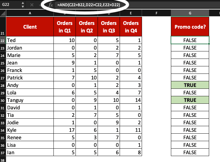
Excel AND function with 3 criteria or more
You’ll see it’s easy to use AND function in Excel for 3 or more conditions.
First, click the cell where you want the result to appear.
Then, enter =AND(condition1, condition2, condition3) and press Enter.
In our example, we want to check if some clients increased the number of orders each quarter. If so, we will send them a promo code to thank them!
condition1 is C>B
condition2 is D>C
condition3 is E>D
If all these conditions are met, the result will be TRUE. If not, FALSE will appear.
In this example, Tanguy and Andy ordered more with us quarter after quarter.
Thanks to Conditional Formatting, it’s easy to see TRUE results!
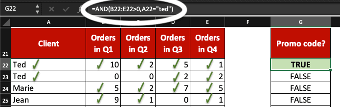
Excel AND function with text: how to write it
Use AND with text elements in Excel by writing text within quotation marks “”.

For example, =AND(B22:E22>0,A22=”Ted”) will be TRUE if cells B22 to E22 contain numbers higher than 0 and cell A22 contains Ted or ted.
To help you understand, if all cells are ticked with a green sign, the result is TRUE. If not, the result is FALSE.
Now, you know how to write the Excel AND function for one or multiple conditions, for one or multiple cells; you also learned how to write AND function with text for the system to check conditions.
New to Spreadsheets? Check out our Excel and Google Sheets Course for $0!