You may use SUMIF instead of VLOOKUP in some cases. If you are not familiar with the SUMIF function in Excel, be confident you will be after reading our tutorial!
What is SUMIF in Excel?
The SUMIF function sums the values in a specific range that meet criteria that you specify.
For example, if you want to know how much you earned from customers who spent over $ 10k, you could use the formula =SUMIF(A2:A30,”>10000″) if amounts are in cells A2 to A30.
SUMIF meaning in Excel
SUMIF means that the system will sum all the values in a specific range if they meet criteria that you specify.
What is the SUMIF formula?
The SUMIF formula is =SUMIF(range, criteria, [sum_range])
SUMIF contains 2 required arguments and 1 optional one ([sum_range]).
range — the range of cells you want to evaluate.
criteria — a criteria defining which cells (within range or sum_range) to add to the sum.
sum_range — this argument is optional but often used. If you want to sum cells in a different range than the one you specified in range, you can do it by specifying where in sum_range. Check our various examples below for more information.
The SUMIF function will result with a number, a sum.
Tips when using SUMIF in Excel
– Enclose text criteria or criteria with logical/mathematical symbols in quotation marks (“text“).
– You may use wildcard characters in the criteria argument. A question mark (?) will search for any single character and an asterisk (*) will match any sequence of characters.
– Sum_range and range should be the same dimensions and shape or your Excel table may be impacted.
How to use SUMIF in Excel?
Learn how to use SUMIF by applying the formula =SUMIF(range, criteria, [sum_range]) and by checking examples below.
Example — SUMIF with text
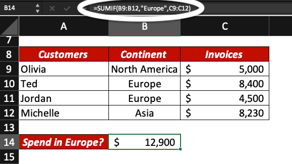
In this example, we use the SUMIF function to know how much European customers are spending with us.
The formula we use is =SUMIF(B9:B12,”Europe”,C9:C12).
Example — SUMIF with text and wildcard characters

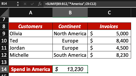
In this example, we use SUMIF to know how much customers from South America and North America are spending with us. Olivia is from North America and Michelle lives in South America. Our criteria is “who lives in America” meaning South or North. We use the wild character * to search for any continents ending with “America”.
The formula we use is our Excel table is =SUMIF(B9:B12,”*America”,C9:C12).
Example — SUMIF with numbers
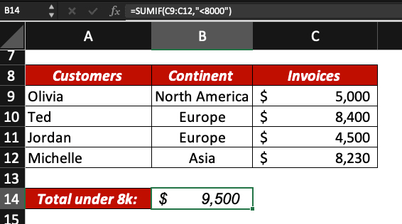
Now, we want to know the sum represented by invoices with an amount inferior to $ 8,000.
The formula we use is =SUMIF(C9:C12,”<8000”). There are 2 invoices with an amount below $ 8,000: 4,500+5,000=9,500.
Example — SUMIF with specific cell

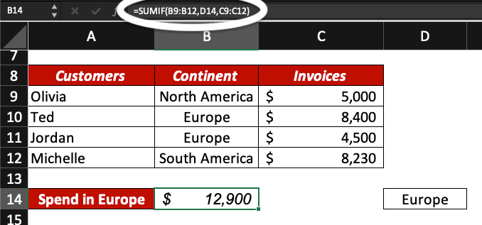
In this example, we want to know how much European customers are spending with us but we are using the cell D14, containing the text “Europe”, as criteria.
The formula we use is =SUMIF(B9:B12,D14,C9:C12).
Now, you know what the SUMIF formula is and how to use the SUMIF function in Excel. For some cases it might be better to use VLOOKUP.
If you want to use SUMIF with multiple criteria, you’ll have to use SUMIFS instead. We’ll explain this slightly different function in a different tutorial. Stay tuned!