Do you want to upgrade your Excel worksheet to the next level? Use dynamic values in Excel text box to give a professional look to your spreadsheet.
What is a dynamic value in Excel?
A dynamic value corresponds to the result of a calculation made within a specific range. If the content within the specific range changes, the value is recalculated automatically. Change the specified range and the value will dynamically update too.
How to mix text values and formulas within a cell?
You can mix text and formulas within the same cell in Excel. Read the steps below to learn how to do it:
- In a cell, type =” and enter the text to want to use. Don’t forget to close with quotations marks.
- Now add an ampersand symbol (&) and enter the formula or function you want to use.
- Press Enter.
Notes
– Note that every time you want to mix text and formulas you will have to add the ampersand symbol (&) between them.
– We do recommend you to add the ROUND function for average calculations in dynamic values in text. Otherwise you may end up with a really long number (see example below “Adding ROUND function“).
Examples
Example of dynamic value – COUNTIF function
If you need to count how many times a value appears within a specific range, you can use the COUNTIF function in Excel.
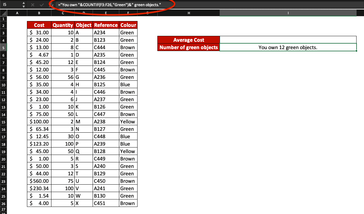
In this example, we decided to highlight how many green objects our client owns. To do so, we are using dynamic value within a text in cell I5.
The formula syntax we used is: =”You own “&COUNTIF(F3:F26,”Green”)&” green objects.”.

In purple you can see the text elements while the COUNTIF formula is highlighted in red. Highlighted in yellow is the ampersand symbol used to link text and function elements together.

Example of dynamic value – SUM function
Use dynamic value in text to showcase average value for example.
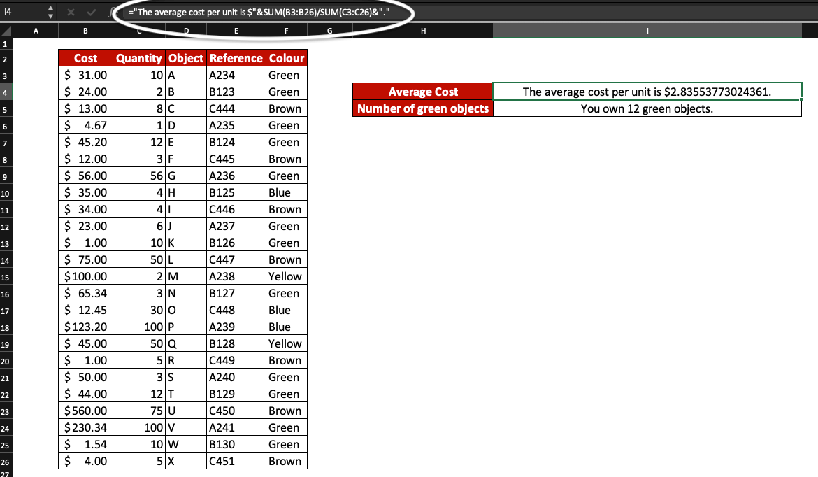
Here, we want to highlight the average cost per object in cell I4. We used this formula: =”The average cost per unit is $”&SUM(B3:B26)/SUM(C3:C26)&”.”

In purple you can see the text elements while formulas are highlighted in red. Highlighted in yellow is the ampersand symbol used to link text and formulas elements together.

You may have noticed that the average price per object contains way too many decimals to look good or to look professional. Use the Excel ROUND function to fix this quickly.
Example of dynamic value – Adding ROUND function
Combine several text and formula elements using dynamic value in text.
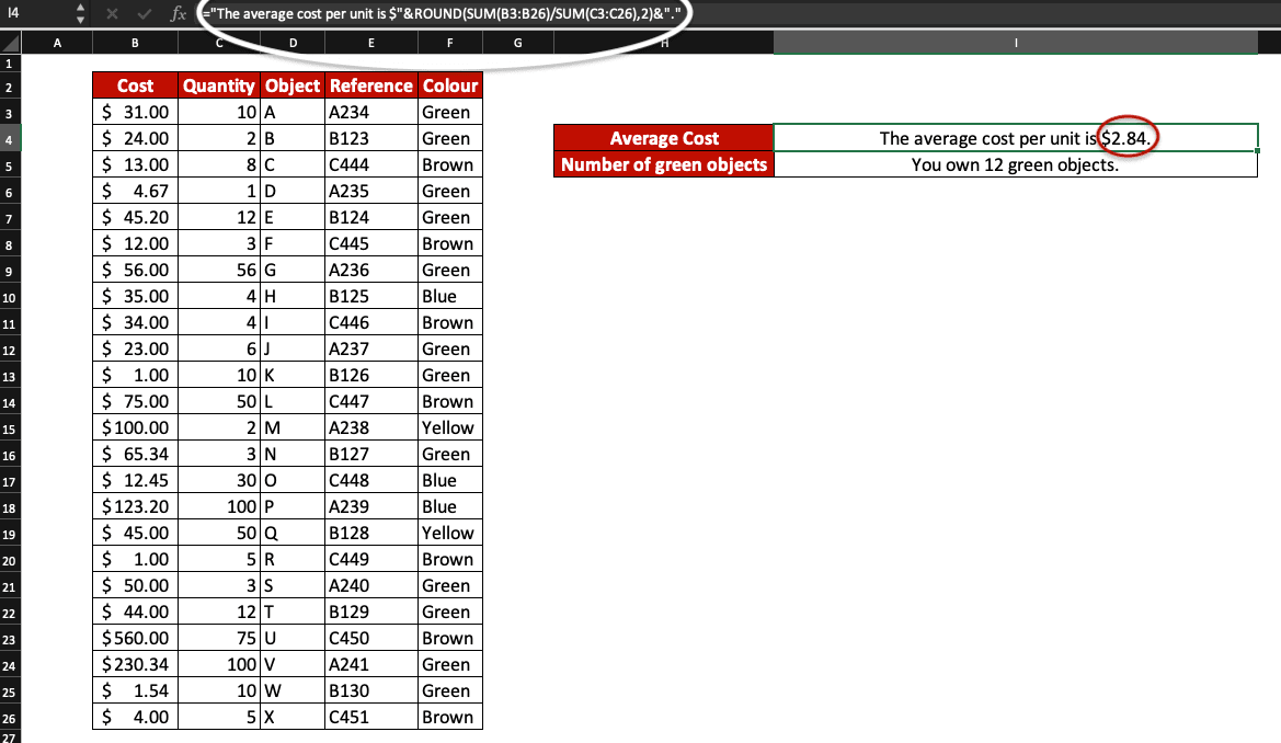
Use the ROUND function if you want to round up or down a number in Excel. In this example, the average cost per unit contains too many decimals so we will round it up to 2 decimals.

We now have a dynamic value in a text with various formulas.
=”The average cost per unit is $”&ROUND(SUM(B3:B26)/SUM(C3:C26),2)&”.”

Now, you know how to use dynamic text values in your Excel worksheets!
Discover more useful tips and tricks by visiting our blog: handy keyboard shortcuts, how to split text into columns, how to add slicers in Excel, how to increase indent, etc.
Limited Offer


