Did you know it’s possible to filter data with a formula in Excel? Instead of using the Filter tool we all know, save time: use the FILTER function.
This Excel function lets you filter with condition: you can add multiple criteria in the formula.
This dynamic filtering feature is really handy when modifying the data you are filtering.
Ready to learn how to use one more Excel formula?
How to filter data with a formula
Instead of using the Filter tool in Excel, use the FILTER formula to dynamically filter data and work more efficiently.
FILTER formula in Excel
The FILTER formula is =FILTER(array,include,[if_empty]) and only array and include arguments are required.
array – the range of cells to filter and display
include – one or more conditions determining the filter criteria
[if_empty] – the value to return if FILTER returns no data
Tips when using the FILTER formula
To avoid unwanted results when filtering data with a formula in Excel, follow these tips:
- Make sure arguments don’t contain errors or the FILTER function will return an error.
- If you want to skip the step mentioned above, use IFERROR.
- Make sure the include argument can be converted to a Boolean value (TRUE or FALSE).
- Use the multiplication operator * to combine 2 conditions in the include argument. This is the equivalent of “and”.
- Use the addition operator + as “or” in the include argument.
- FILTER is not case sensitive so remember this if letter case is a differentiating criteria.
- Lock ranges (use the dollar sign $) when using the FILTER formula in different columns or rows.

How to filter with condition in Excel?
Filter your data with the FILTER formula in Excel and add conditions in the include argument. For example, =FILTER(A1:D10,C1:C10=”excel”) will return rows if the data in the corresponding cell C only contains the text “excel” (in lowercase or uppercase letters).
Check the examples below to get familiar with the FILTER formula in MS Excel.
Filter data with a formula: examples with FILTER
Filter your data with 1 or 2 conditions using the FILTER formula. Accustom yourself with the Excel FILTER function, check the following examples!
Filter data – one condition or the other
Filter out data based on one criteria or the other using this formula template =FILTER(array,(criteria1)+(criteria2),[if_empty] (as a reminder, [if_empty] is optional).
In this example, we want to know when Ted or Jordan were managing projects based in our data. The formula we use is =FILTER(A17:A28,(C17:C28=”ted”)+(C17:C28=”jordan”))
Remember that the FILTER formula is showing results dynamically: if you modify the filtered data, results will be updated. Isn’t it great?

Filter data dynamically – two conditions
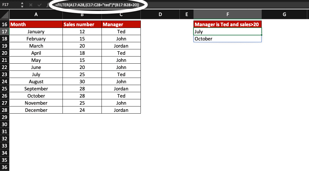
To filter data based on two conditions (or more), use this formula template: =FILTER(array,(criteria1)*(criteria2),[if_empty]

In this example, we want to know when Ted was the manager and sales number were higher than 20. The FILTER formula we use is =FILTER(A17:A28,(C17:C28=”ted”)*(B17:B28>20))
We did not use the optional argument [if_empty].
Filter data in multiple columns
Finally, if you wish to use the FILTER formula in multiple columns, for example, you may need to lock some ranges of cells. To do so, use the dollar sign $.
Discover how to lock cells instantly with this shortcut!
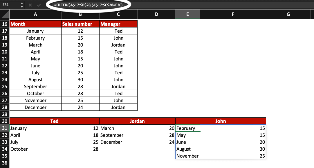
In this example, we want to highlight the number of sales per month for each manager and decide to split the results per manager.
The FILTER formula we use in cell A31 is =FILTER($A$17:$B$28,$C$17:$C$28=A30) for Ted; the system applies automatically changes to A30 (becoming B30 for Jordan and E30 for John) when we paste the formula in cells C31 and E31.
Now, you know how to filter data with a formula in Excel, how to use conditions to filter data and how to lock cells using a handy shortcut.
Learn how to create impressive dashboards in Excel and Google Sheets: join our free online course now!