Merge cells in Excel without losing data with these 3 simple methods: Ampersand, CONCAT and CONCATENATE.
Learn how to use different ways to concatenate text in Excel, to merge cells, to combine two columns or more.
Time to become an Excel Master!
Are you ready to learn new Excel tips and tricks today?
How to concatenate in Excel
Concatenate in Excel is pretty simple and can be done in various ways. Use the handy CONCAT and CONCATENATE formulas or use the Ampersand symbol to combine cells data.
First, we’ll explain what CONCAT and CONCATENATE functions are and what is the difference between these two Excel functions. Then, we’ll show you how to use Ampersand (&) to merge data from two or more cells in Excel.
Of course, examples will be shared with you so you can familiarise yourself with these new Excel formulas and tricks.
CONCAT vs CONCATENATE
What’s the difference between CONCAT and CONCATENATE in Excel? How to use these functions? What are the formulas?
Find the answers to these questions below!
CONCATENATE function
Use CONCATENATE to combine two columns or more or various cells. This Excel function allows you to join cells content (text, number, reference) without losing any data.
The CONCATENATE formula is =CONCATENATE(text1, [text2],…) and you can join up to 255 arguments. Use quotation marks (“”) to wrap text elements; numbers don’t need to be wrapped.
text1 – the 1st data to combine.
[text2],…– other cells or text strings you want to combine with text1.
Excel CONCAT function
The CONCAT function works exactly as CONCATENATE in Excel: this function replaces CONCATENATE. There is no difference between CONCAT and CONCATENATE in Excel.
Note that CONCATENATE is still available for now for compatibility reasons. We do recommend you to use CONCAT instead, in case CONCATENATE disappears in the future.
The CONCAT formula is =CONCAT(text1, [text2],…) and its arguments work as previously explained with CONCATENATE.
text1 – the 1st data to combine.
[text2],… – other cells or text strings you want to combine with text1.
Again, use quotation marks (“”) to include text elements or symbols in your arguments.
Combine cells with Ampersand
In your worksheet, you can use Ampersand (&) to combine data instead of CONCAT and CONCATENATE.
We already mentioned this symbol and its use in tutorials such as this one: How to find UNIQUE values in Excel?
Combine cells data with Ampersand by following this formula: =”text1″&”text2″&”text3″…
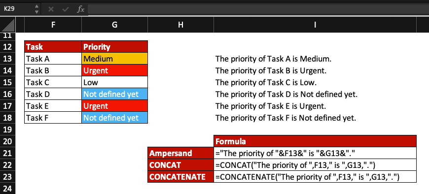
For example, let combine two columns with Ampersand without losing any data: columns F and G.
Here, we want to merge cells F and G so we can read in column I a phrase like “The priority of Task A is Medium.”
The formula we use is =”The priority of “&F13&” is “&G13&”.”
We could add the LOWER function to change the content in G13 to lower case. The formula would be =”The priority of “&F13&” is “&LOWER(G13)&”.” and the result “The priority of Task A is medium.“

How to concatenate two columns in Excel
Familiarise yourself with CONCAT and CONCATENATE in Excel by checking the examples below, where we combine data from two columns.
Merge cells with CONCAT
In this example, we want to combine cells in Excel using the CONCAT function.
Let merge cells from two columns (F and G) so the result in column I is “The priority of Task A is Medium.”
The CONCAT formula we use is =CONCAT(“The priority of “,F13,” is “,G13,”.”)

We mentioned before that CONCAT is replacing CONCATENATE but if you want to use this latter function, learn how to use it below.
Merge cells with CONCATENATE
We use the same example as per above: we want to combine cells data from two columns (F and G).
The CONCATENATE formula we use, for the same result, is =CONCATENATE(“The priority of “,F13,” is “,G13,”.”)

You have seen 3 examples where cells data were combined using CONCAT, CONCATENATE and Ampersand. 3 different ways for the same result!

Now, you know how to combine cells in Excel without losing data! You discovered 3 ways of joining cells and that there is no difference between CONCAT and CONCATENATE.
Which one of these 3 methods will you pick next time?


