HLOOKUP vs VLOOKUP for dummies: Excel formulas and examples

Most of us have heard about the VLOOKUP function, but not so much about HLOOKUP in Excel. Today, learn the difference between these two handy formulas and how to use them in your spreadsheets.

In this tutorial, you’ll find formulas, tips, examples for HLOOKUP and VLOOKUP.

VLOOKUP for dummies

What does VLOOKUP stand for?

VLOOKUP stands for Vertical LOOKUP. This Excel function is useful when you need to find an information by row, within the same sheet or within another one, in a specific array of columns.

Tips when using Vertical Lookup

• Make sure the return value is on the right side of the column you search from.
• We recommend using 0 as the range_lookup argument, to avoid unwanted results.
• You can use wildcard characters in the lookup_value argument if range_lookup is 0/FALSE and lookup_value is text. A question mark (?) will search for any single character and an asterisk (*) will match any sequence of characters.
• Return value will be 0 in Excel if the cell containing the return value is empty. If the cell containing the value you need is a formula, the return value will be the result of the formula.

VLOOKUP examples in Excel

Searching a value within the same worksheet – reference

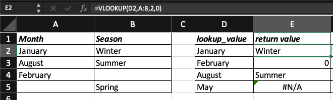
In this example, we want to find the season (value to return) associated to the month mentioned as lookup_value; lookup_value is a reference (D2, D3, etc.).

Searching a value within the same worksheet – specific value

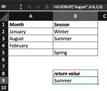
In this example, we want to find the season (value to return) associated to the month of August; lookup_value is a specific value (“August”).

Searching a value within the same worksheet – wildcard

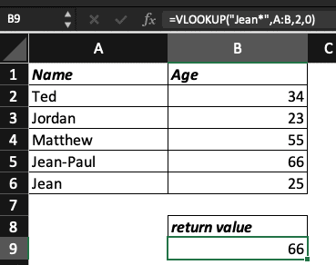
In this example, we want to know the age of Jean-Paul but we don’t want to write his name entirely to save time; lookup_value is a specific value. We are using the wildcard *.

Using VLOOKUP between two sheets

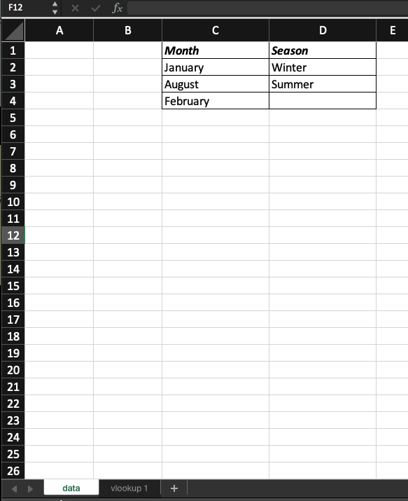
In this example, we want to find the season (value to return) associated to the month mentioned as lookup_value; lookup_value is a reference. The data is on the sheet “data”.

The Excel sheet with the data we need:

The Excel worksheet with our VLOOKUP formula:

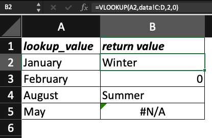
The VLOOKUP formula we used is =VLOOKUP(A2,data!C:D,2,0). Explanations:

• A2 – the reference of lookup_value.
• data!C:D – the value to return is in the sheet named data and the columns we need are columns C and D. In column C, we have the lookup_value and in column D the value to return.
  Again, the value must be in the 1st column of the range of cells selected as table_array so we could not select data!A:D as table_array in this example.
• 2 – the value to return is in column number 2.
• 0 – we want an exact match.

What is HLOOKUP?

What does HLOOKUP stand for?

HLOOKUP stands for Horizontal Lookup. The HLOOKUP function searches for a value in the 1^st row of a table and returns a value in the same column, from any row you specify.

How to use HLOOKUP in Excel

In Excel, the HLOOKUP function includes 4 arguments: 3 are required and 1 is optional (range_lookup).

The HLOOKUP formula is: =HLOOKUP(lookup_value, table_array, row_index_num, [range_lookup])

• lookup_value – the value you want to find.
  The value must be in the first row of the table or array you select.
• table_array – the range of cells in which the lookup_value and the return value you want to find are.
• row_index_num – the row number where the return value is, within your table_array.
  The first row within your table_array is number 1.
• range_lookup – logical value specifying if you want the HLOOKUP function to find an exact match (0/FALSE) or an approximate one (1/TRUE).
  If you don’t specify this argument, the default value is always 1/TRUE.

HLOOKUP Tips

• We recommend using 0 as the range_lookup argument, to avoid unwanted results.
• Make sure the return value is below the row you search from. HLOOKUP can’t look upward!
• The value in the lookup_value argument can be a text, a formula or a reference.
• The return value will be 0 in Microsoft Excel if the cell containing the return value is empty. If the cell containing the value you need is a formula, the return value will be the result of the formula.
• Like for the VLOOKUP function, with HLOOKUP, you can use wildcard characters in the lookup_value argument if range_lookup is 0/FALSE and lookup_value is text. A question mark (?) will search for any single character and an asterisk (*) will match any sequence of characters.
• Uppercase and lowercase text values are equivalent.

HLOOKUP examples

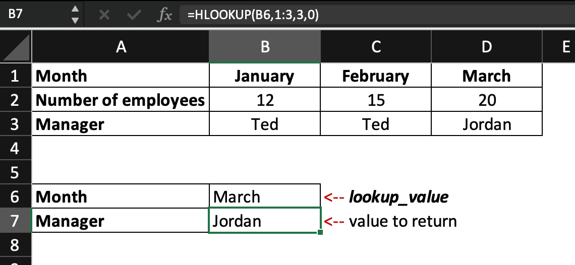
Searching a value within the same table – reference

In this example, the lookup_value is a reference, the cell B6 mentioning the month of March.

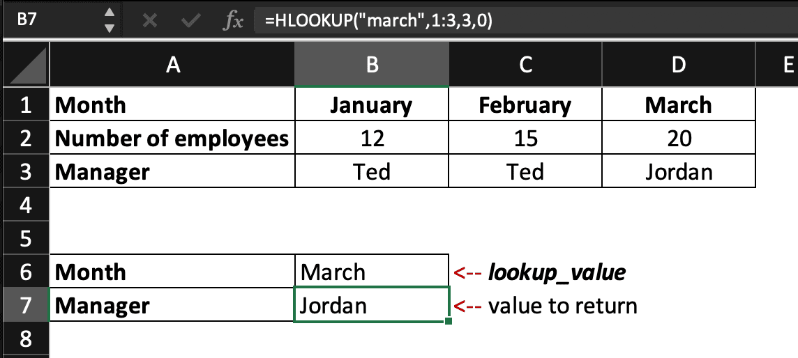
Searching a value within the same table – specific value

In this example, the lookup_value is a specific value (March). For texts, lowercase or uppercase values are equivalent so, here, the lookup_value can be written “March” or “march”.

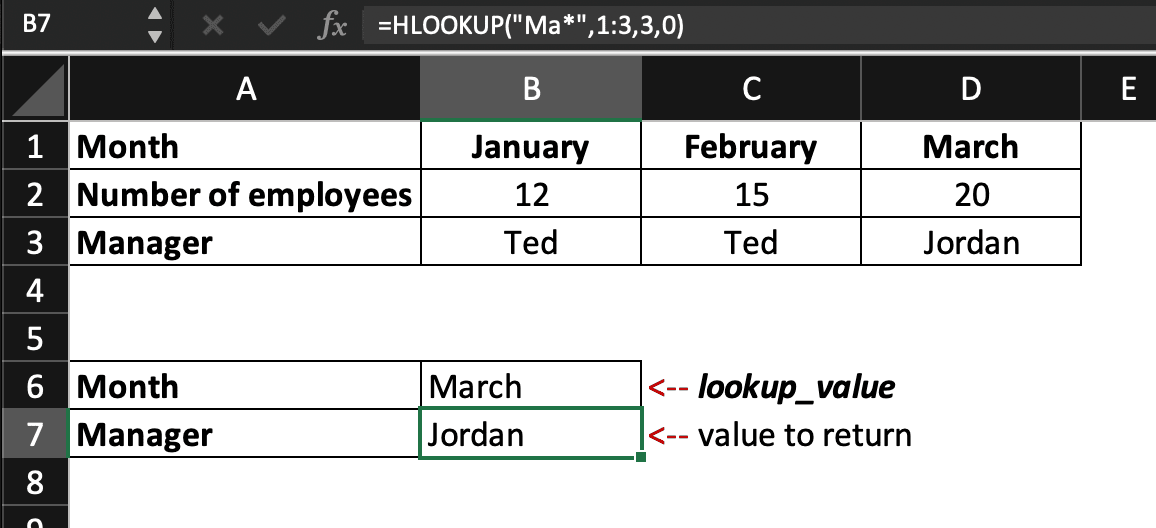
Searching a value within the same worksheet – wildcard

In this example, we are using the wildcard character * to save time: we know that only the month of March starts with M in English. We could use “M*” as lookup_value but in our example, we add “Month” within the table_array so we have to be a bit more specific to avoid any unwanted results.
If we wanted to find the name of the manager in charge during February, we could use “F*” as lookup_value to save time.

HLOOKUP vs VLOOKUP

Now you know that VLOOKUP stands for Vertical Lookup and that HLOOKUP stands for Horizontal Lookup. You understand the difference between these two Excel functions and when to use one or the other.

VLOOKUP helps you search for a value in the first column of a table array and returns a value in the same row, from any column you specify. HLOOKUP, on the other end, helps you find a value in the first row of a table and returns a value in the same column, from any row you specify.

If you want to learn how to use other handy Excel formulas and tools, check out our Spreadsheet Online Course! You’ll receive an Excel certification to add to your resume or to your LinkedIn profile page.

You might have noticed that, sometimes, the result of the VLOOKUP formula was N/A… Learn how to change N/A to a nicer result by using the IFNA function.

I you liked our free Excel tutorial for dummies and beginners, feel free to share it!